The Simplest Example of Gradient Descent
create data first
x = [338., 333., 328., 207., 226., 25., 179., 60., 208., 606.]
y = [640., 633., 619., 393., 428., 27., 193., 66., 226., 1591.]
import numpy as np
import matplotlib.pyplot as plt
# y = b + w*x
# initial the parameters
b = -120
w = -4
learning_rate = 0.0000001
iteration = 100000
# store the iteration value for plotting
b_history = []
w_history = []
# iteration
for i in range(iteration):
    b_gradient = 0.0
    w_gradient = 0.0

    for n in range(len(x)):
        b_gradient = b_gradient - 2.0 * (y[n] - b - w*x[n])*1.0
        w_gradient = w_gradient - 2.0 * (y[n] - b - w*x[n])*x[n]

  # update parameters
    b = b - learning_rate * b_gradient
    w = w - learning_rate * w_gradient

    b_history.append(b)
    w_history.append(w)
Plot the result
x_plot = np.arange(-200, -100, 1) #bias
y_plot = np.arange(-5, 5, 0.1) #weight
Z = np.zeros((len(x_plot), len(y_plot)))
X, Y = np.meshgrid(x_plot, y_plot)
for i in range(len(x_plot)):
    for j in range(len(y_plot)):
        b = x_plot[i]
        w = y_plot[i]
        Z[j][i] = 0
        for n in range(len(x)):
            Z[j][i] = Z[j][i] + (y[n] - b - w*x[n])**2
        Z[j][i] = Z[j][i]/len(x)
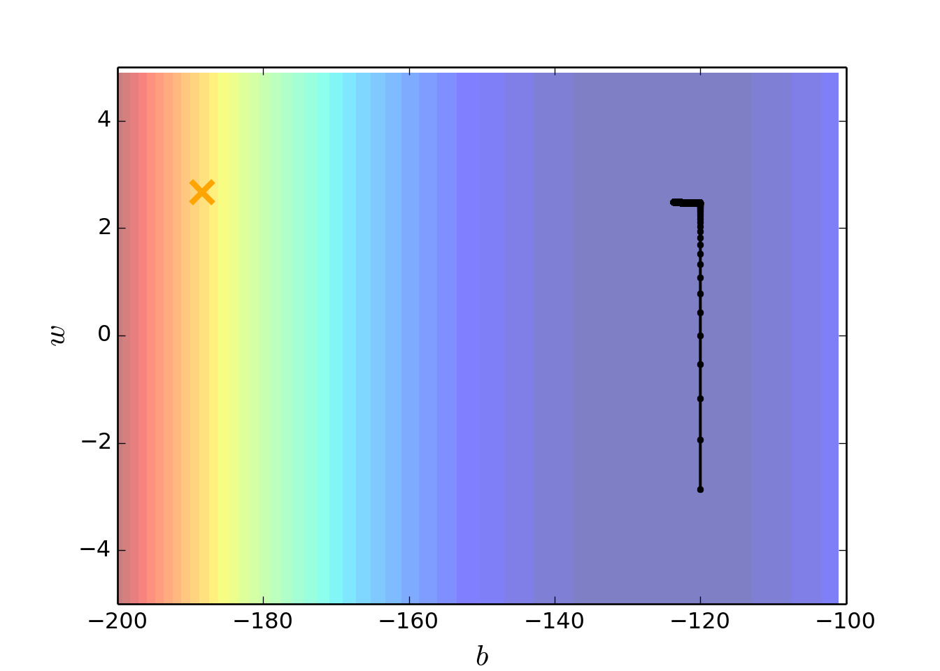
plt.contourf(x_plot, y_plot ,Z, 50, alpha = 0.5, cmap = plt.get_cmap('jet'))
## <matplotlib.contour.QuadContourSet instance at 0x1122283f8>
plt.plot([-188.4], [2.67], "x", ms = 12, markeredgewidth = 3, color = "orange")
plt.plot(b_history, w_history, "o-", ms = 3, lw = 1.5, color = "black")
plt.xlim(-200, -100)
## (-200, -100)
plt.ylim(-5, 5)
## (-5, 5)
plt.xlabel(r'$b$', fontsize =16)
plt.ylabel(r'$w$', fontsize =16)
lecture from: Hung-yi Lee